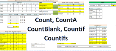
Excel to use Count, CountA, CountBlank, Countif, Countifs..

How to use Count and other functions

"Thanks you everyone for your response. Today we are going to discuss the use of Count, CountA, CountBlank, Countif, Countifs..,  basically these are very simple functions but very important. They are used mostly to count something specific within a range. Only issue with these functions they are not used completely with arrays. There are some limitations.

 

 

 

 

 

 

 

 

 

 

Lets start:-

• Count:- Only Count numbers.

• CountA:- Count non blank cells.

• CountBlank:- Count blank cells.

• Countif:- Count based on single condition.

• Countifs:- Count based on multiple conditions.

 

 

It can be used to get the result based on conditions.

 

 

 

 

 

 

 

 

 

Also if you want to test for more than 1 conditions.

 

 

 

 

 

 

 

 

 

You can use it to find out duplicate and unique records.. 

 

Here you can fill the form and the file will be sent to you.

                 AutoMateSheets                     

Directly understand Indirect..

Excel Indirect

"Thanks you everyone for your response. Today we are going to discuss the use of INDIRECT, most of the time you can not use it alone because it just create text into the ranges. So when to use, whenever you are working with the dynamic ranges. You can say it is the synonym of dynamic range in excel. Here we are going to explore it a more and understand the uses of this functions.. 

 

 

 

 

 

 

 

 

 

Lets start  :)

• Indirect -Convert text to range if text is valid range .

•  Syntax
1. ref_text = Enter the cell reference..
2. False or True = Option to select range style.
   
• False = R1C1 style (R3C4)
• True = A1 style (A5)
  

First Example..

•  You  can use for dynamic data validation, where you can create dependent list and use indirect in the validation.

• Company is the first dynamic list which has list as following
• Apple, Google, Microsoft 

• If you see Apple and other companies has list of product so the list is like company name again the product list
• Apple = iPhone, Mac, iPad
• Google = Pixel, Google Glass, Chromecase
• Microsoft = Lumia, Surface, Xbox

Now if you use indirect(Company) it will bring the first list in the cell where you will apply the validation, for example A1.

If you go to A2 and create data validation again the above mentioned cell like, indirect(A1)..boom.. you will get the product list here and whenever the first list changes the second list will also change.

Here you can fill the form and the file will be sent to you.

                                     AutoMateSheets                                  

 

 Here is the YouTube video, where I have explained everything..

Please get in touch for any query help or suggestion..
Youtube
Facebook Page
Twitter
Email: lkthecool@gmail.com

Excel Vlookup and Hlookup

Vlookup & Hlookup

"Thanks you everyone for your response. Today we are going to discuss basic lookup functions Vlookup & Hlookup. Here I want to mention that you can use Index + Match instead of Vlookup & Hlookup since Index + Match has no restriction when you looking up data left to right and down to up. In the practical scenarios when you are in office you see most of the time data in the format where you can use Vlookup (I am not denying that you do not use Hlookup but its very rare)."

"I have seen people who do not know any function but they learnt the Vlookup and use it on daily basis in day to day work, although do not use them for complex problems but it works most of the time for them."

 

Lets start the functions :)

 

• VLOOKUP -Lookup the value in the left most column and extract value from the required column within the data range.

•  Syntax
1. lookup_value - Value you want to match
2. table_array - Range of data set (lookup value should be in first column
3.  col_index_num - Result column
4.  [range_lookup] - Optional (Approximate match-TRUE, Exact match-FALSE)

• HLOOKUP -Lookup the value in the left most column and extract value from the required column within the data range.

•  Syntax
1. lookup_value - Value you want to match
2. table_array - Range of data set (lookup value should be in first column
3.  row_index_num - Result row
4.  [range_lookup] - Optional (Approximate match-TRUE, Exact match-FALSE)

Here is the sample file you can use it to practice where I have created some of the samples..

                     Download workbook

 Here is the YouTube video, where I have explained everything..

Please get in touch for any query help or suggestion..
Youtube
Facebook Page
Twitter
Email: lkthecool@gmail.com

Excel Logical and Information Functions

Logical & Information Functions

"Thanks you everyone for your response. Today we are going to discuss Excel's Logical & Information  functions. "

 

Before you start: Excel has only 2 logical statement TRUE and FALSE (this is different from if you type them as a text, means just put apostrophe before true or false). In excel True =1 and False =0.
So basic understand is that every logical condition will only return you either TRUE or FALSE, if not you would get the error as a output. If function can take advantage of any information formulas since if has the ability to show output based on condition/s :) 

 

Lets start the functions :)

• IF- Based on the logical test (True / False) allow user to show output. 

• AND - Returns TRUE if multiple condition are true. 

• OR- Returns TRUE if any argument is TRUE. 

• XOR - Returns TRUE, if 1 condition is true and 2 is false or vice versa. If both True and False it shows as false. If you take more then 2 arguments then results would be depends on number of conditions (either odd or Even then return True or False).

• TRUE - Logical value (if you simple put in 1st argument of if, your True part will be executed). 

• FALSE- Logical value (if you simple put in 1st argument of if, your False part will be executed).

• NOT - Reverse the logic of any logical test (Not(False) is same as True). 

• IFERROR - Error the handles and if error occurs in statement then it will show the next user defined output.  

• ISBLANK - Returns TRUE if the value is blank.

•  ISERR - Returns TRUE if the value is any error value except #N/A.

• ISNA - Returns TRUE if the value is the #N/A error value.

• ISERROR - Returns TRUE if the value is any error value.

• ISEVEN - Returns TRUE if the number is even.

• ISODD - Returns TRUE if the number is odd.

• ISLOGICAL - Returns TRUE if the value is a logical value.

• ISREF - Returns TRUE if the value is a reference.

• ISNUMBER - Returns TRUE if the value is a number.

• ISTEXT - Returns TRUE if the value is text.

• ISNONTEXT - Returns TRUE if the value is not text.

Here is the sample file you can use it to practice where I have created some of the samples..

                     Download workbook

Here is the YouTube video, where I have explained everything..

Please get in touch for any query help or suggestion..
Youtube
Facebook Page
Twitter
Email: lkthecool@gmail.com

Excel Date & Time Functions

Date & Time Functions

"Thanks you everyone for your response. Today we are going to discuss Excel's Date & Time functions. These functions are really important because it is most common that you would have date & Time in your data and you want to extract some meaningful information.

 

Lets start the functions :)

• TODAY - Returns the serial number of today’s date. 

• NOW - Returns the serial number of the current date and time (time is not there when you use Today). 

• DAYS360 - Calculates the number of days between two dates, based on a 360-day year. 

• EDATE - Returns the serial number of the current date and time. 

• EOMONTH - Converts a serial number to a day of the month. 

• NETWORKDAYS- Returns the number of whole workdays between two dates. 

• WEEKNUM - Returns the week number in the year. 

• WORKDAY - Returns the serial number of the date before or after a specified number of workdays. 

• Datedif- Show you differene between 2 dates, using multiple criteria.

• This function does not show up automatically, the intelisense feature does not work for this. you need to type it exactly like this.

•  DAY- Converts a serial number to a day of the month.

• MONTH- Converts a serial number to a month.

• YEAR - Converts a serial number to a year.

• DATE - Returns the serial number of a particular date.

• HOUR- Converts a serial number to an hour.

• MINUTE - Converts a serial number to a minute.

• SECOND - Converts a serial number to a second.

• TIME- Returns the serial number of a particular time.

• DATEVALUE- Converts a date in the form of text to a serial number.

• TIMEVALUE - Converts a time in the form of text to a serial number.

Here is the sample file you can use it to practice where I have created some of the samples..

                     Download workbook

Here is the YouTube video, where I have explained everything..

Please get in touch for any query help or suggestion..
Youtube
Facebook Page
Twitter
Email: lkthecool@gmail.com

Excel String/Text functions with examples..

Basic Text Functions

"Thanks you everyone for your response. Today we are going to discuss Excel's strings / text functions. These functions will help you create a strong base. I am not saying you always need them but if you know them you can definitely work faster in Excel."

Lets start the functions :)

• LEFT - Take out specific number of characters from the left. 

• MID - Take out specific number of characters from Middle (can be left or right as well).

• RIGHT - Take out specific number of characters from the Right.

• FIND - Find any specific text, within text (case sensitive)

• SEARCH - Find any specific text, within text (not case sensitive).

• SUBSTITUTE - It changes text to some other text provided by user.

• REPLACE - It changes text to some other text provided by user.

• TEXT - It take cares all the formats you want in Excel.

• REPT - It repeats the characters.

• CONCATENATE - Merge text or numbers, It was concatenate but new excel version has been changed to concat.

• CODE - Converts value to code/Asc.

• CHAR - Converts value to char/chr.

• NUMBERVALUE / VALUE - Convert text into numbers.

• PROPER - Make strings to proper case

• UPPER - Make strings to upper case

• LOWER - Make strings to lower case

•  TRIM - Remove extra space.

• CLEAN - Clean data, remove non printable characters

• DOLLAR - Put a dollar symbol before the numbers.

• T - Test whether you have test or number.

• EXACT - Compare binary formats (case sensitive).

• LEN - Count the length of a text or number.

Here is the sample file you can use it to practice where I have created some of the samples.

                            Download File...

Here is the Youtube video, where I have explained everything..

 

Please get in touch for any query help or suggestion..
Youtube
Facebook Page
Twitter
Email: lkthecool@gmail.com

Index + Match - Together they can find any thing..

Index + Match 

 

Thanks you all for your response and again coming here... 

I really got a good response on offset so I thought to explore Index + Match. If you want to follow me, click on Follow me.

Index Match for Images-

Lets talk about one by one so you understand there is no practical use, if you use any of them alone.

Index

There are 2 versions of Index and we will talk about the first one only.

1. Index(array,row_num,[column_num]) 
2. Index(reference,row_num,[column_num],[area_num])

Syntax

• Array - This is a range, it can have both rows or columns. It depends on your data set, see example below-
• A1:A10 - only rows
• A1:J1 - only columns
• A1:J10 - rows + columns  

•  row_num - If you have selected 4 rows for example and you want to take out the row number 2 data then this argument will be 2.
• column_num - If you understand the above one then it is the same logic. If you have selected 3 column and you want to take out column 2 data then this argument will be 2.

Note: In this formula column_num is optional but this is not the case, row_num can also be optional if you put the column_num value and leave the row field blank then system will always show you 1st row data and same applies with column.

Basic understanding - Quite clear, how Index work and you can get the data from array by passing arguments row number and column number.
Ok lets think again, does it make any sense when you are entering numbers manually..Noooooo.
If you already know what data you want to extract you can do it manually. Now this function
has no worth, absolutely right in this way but wait just have some info about Match.

Match

• Match(lookup_value,lookup_array,[match_type])

Syntax

• lookup_value -As simple as that, what you want to search (any string, any number).
• lookup_array - It is same as Index array but there is difference either you can select rows or the columns. You can not combine them.
• match_type -You can put 3 inputs type -1,0,1. For exact match you should enter 0 only, most of the times exact match is used. To know more about this click on Excel Lookup Functions.

Basic understanding - Again no use of this formula, it only gives you the sequence number not the lookup value or in other words it tells you exact position of the lookup value. What will you do with the sequence number. Here comes the Index and Match relationship.

We just talk about Index row_num and column_num, so these are the 2 arguments that can be passed by entire match function (which give you the sequence number). Now you can really explore the power of Index + Match.

Index + Match Example

Thanks for reading all this, I will soon upload the video on you tube.

Please get in touch for any query help or suggestion..
Youtube
Facebook Page
Twitter
Email: lkthecool@gmail.com